AP Statistics Notes — 2026–27 Study Guide
Scope: This five-unit review uses College Board’s 2026–27 framework, first examined in May 2027. It is algebra-based and does not require calculus. School pacing can differ. If you use an older nine-unit guide, compare topics rather than matching unit numbers. The current framework excludes geometric distributions, combining random variables, chi-square goodness-of-fit tests, and inference for regression slopes. Two-way-table chi-square tests and descriptive regression remain relevant. Transforming nonlinear models is outside this review.
Scope: The five PART sections follow the current five-unit structure. School pacing can differ. If you use an older nine-unit guide, compare topics rather than matching unit numbers. The current framework excludes geometric distributions, combining random variables, chi-square goodness-of-fit tests, and inference for regression slopes. Two-way-table chi-square tests and descriptive regression remain relevant. Transforming nonlinear models is outside this review.
Symbols used: n = sample size; N = population size; x̄ and s = sample mean and sample standard deviation; μ and σ = population mean and standard deviation; p̂ = sample proportion; p = population proportion; SE = standard error. In a test, H₀ is the null hypothesis and Hₐ is the alternative. A star, as in z* or t*, marks a critical value.
References: College Board course framework, effective Fall 2026, course and exam revisions, and current exam information. Scope and exam facts were checked on October 16, 2026. All data sets and practice questions below are invented for teaching.
How to use this review
If this is your first encounter with a topic, use the matching lesson from your teacher or course alongside these notes. Start with the PART for that topic and work through its examples. For revision, attempt that PART’s checkpoint first; use any missing step to decide what to reread.
For one study session: read one PART, cover a worked solution and reproduce it, then try the checkpoint without the notes. Appendix B contains worked answers and a self-check list. Explain a result in words as well as calculating it. Getting the arithmetic right while choosing the wrong method is still a gap to revisit.
The quiz follows the same order: Unit 1 uses Q1–5; Unit 2 Q6–10; Unit 3 Q11–17; Unit 4 Q18–21; Unit 5 Q22–25. These small sets are practice samples, not a pass/fail rule for a unit. Keep a record of missed methods or interpretations, and try those items again after a gap without consulting the answer.
PART 1 — EXPLORING ONE-VARIABLE DATA AND COLLECTING DATA
1.1 Begin with a question and a population
A statistical investigative question identifies a group and a variable and anticipates variation. “How long do students at this school spend on homework on a typical weekday?” invites a distribution of answers. “How many minutes did Maya study yesterday?” asks for one person’s value rather than a pattern across a population.
The population is the entire group the question concerns. The sample is the group actually observed. A parameter describes a population, such as the proportion of all students who use the library. A statistic describes a sample, such as the proportion among 200 sampled students. Define the population, measurement unit, time period, and operational meaning of the response before collecting data.
A categorical variable assigns labels, such as travel mode. A quantitative variable records a meaningful numerical amount, such as travel time in minutes. A numeric student ID is still a label; averaging IDs has no useful interpretation.
1.2 Choose and describe displays
For one categorical variable, use a frequency or relative-frequency table, a bar chart, or a pie chart with a meaningful whole. For one quantitative variable, use a dotplot, stemplot, histogram, or boxplot. Histogram bars represent numerical intervals; bar-chart bars represent categories. A cumulative relative-frequency graph helps locate percentiles, while a boxplot highlights quartiles and potential outliers but hides some distribution detail.
Describe quantitative distributions in context: shape, center, spread, and unusual features. Compare groups with explicit comparative language, such as “Group A has a larger median and a wider interquartile range.” Right skew means the long tail points toward larger values; it does not mean most observations are large.
The median is the 50th percentile; Q₁ and Q₃ mark the lower and upper quartiles, associated with the 25th and 75th percentiles. For the small samples in these exercises, take the median of each ordered half; when n is odd, leave the overall median out of both halves. Quartile algorithms can differ, so use a question’s stated convention.
The mean uses every value and is sensitive to extreme values. The median depends on order and is more resistant. Pair the median with the interquartile range (IQR) for a skewed distribution; the mean and standard deviation are often useful for roughly symmetric data without influential extremes. A potential outlier falls below Q₁ − 1.5 × IQR or above Q₃ + 1.5 × IQR. Investigate such a point before deciding what to do with it; the rule does not authorize deleting valid observations.
Worked example 1 — Describe a small sample. Five recorded waiting times are 2, 4, 4, 6, and 9 minutes. Their sum is 25, so x̄ = 5 minutes, while the median is 4 minutes. The squared deviations from the mean total 9 + 1 + 1 + 1 + 16 = 28. The sample variance is 28/(5 − 1) = 7 minutes squared, and s = √7 ≈ 2.646 minutes. Dividing by 5 instead would describe the variance of these five values treated as a complete population, not the sample variance.
A standardized score tells how far a value is from a mean in standard-deviation units: z = (x − μ)/σ. A value of 80 in a population with mean 70 and SD 5 has z = 2: it is two SDs above the mean. Standardizing does not make a skewed distribution normal. Adding a constant shifts the center without changing spread; multiplying by a constant multiplies SD and IQR by its absolute value.
Read an actual distribution
The two groups below each contain 20 invented waiting times. Equal bin widths and the same vertical scale make the distributions comparable.
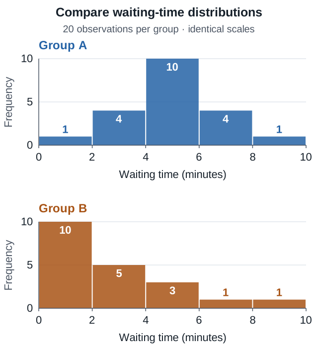
The exact observations are specified by this frequency table; each waiting time is repeated the stated number of times:
| Waiting time (minutes) | 1 | 3 | 5 | 7 | 9 |
|---|
| Group A frequency | 1 | 4 | 10 | 4 | 1 |
| Group B frequency | 10 | 5 | 3 | 1 | 1 |
Describe before calculating: A is approximately symmetric, while B has a long right tail. A’s median is 5 minutes; B’s median is (1 + 3)/2 = 2 minutes. B’s mean is 56/20 = 2.8 minutes, above its median, which is consistent with its right tail. In a histogram, the tail’s direction describes the shape; the tallest bar alone does not describe the whole distribution. These small examples illustrate interpretation and do not justify an inference about real populations.
1.3 Sampling, bias, and ethical collection
In a simple random sample of size n, every possible group of n population members has the same chance of selection. A practical implementation labels the population, uses a random-number generator to select distinct labels, and contacts those selected. Explain what happens to duplicates and how nonresponse is recorded; replacing unavailable people with convenient volunteers can change the design.
- Stratified random sampling: divide the population into relevant groups and randomly sample within every group. This can improve precision and representation when the groups differ on the variable of interest.
- Cluster sampling: randomly select groups and observe all members of those selected groups. It can reduce collection costs; similarity within clusters can reduce precision.
- Systematic sampling: use a random starting point and select at a fixed interval. Check that a recurring population pattern does not align with the interval.
- Convenience or voluntary-response sampling: selection favors available people or those motivated to respond. A large sample alone does not remove that bias.
Undercoverage omits part of the target population. Nonresponse occurs when selected individuals do not provide data. Response bias can arise from leading wording, memory errors, interviewer effects, or sensitive questions. Distinguish nonresponse from voluntary response: one loses selected people; the other lets people select themselves into the sample. Protect consent and privacy, and do not treat misleading survey wording as an acceptable design shortcut.
1.4 Experiments and the scope of a conclusion
An observational study records existing choices or characteristics. A randomized experiment assigns treatments. Confounding makes it difficult to separate the effects of explanatory variables on a response.
A useful experiment identifies experimental units, explanatory factors and treatment levels, a response, and an appropriate comparison. Randomly assign units to treatments, keep other conditions comparable, and use enough independent units to see effects amid variation. A placebo can support a fair comparison when appropriate. Blinding limits expectations; double blinding keeps both subjects and those evaluating responses unaware of assignments where feasible.
Use a randomized block design when a measured characteristic predicts the response: form similar blocks, then randomize treatments within each block. Matched pairs are a special case, such as two measurements on the same person or two closely matched people. When possible, randomize treatment order in a repeated-measures design to reduce order effects.
Worked example 2 — Sampling versus assignment. A school randomly selects 80 students from its roster, then randomly assigns 40 to each of two review schedules. Common testing conditions and a consistent response measure support comparison. Random selection supports generalizing to that school’s students; random assignment supports a causal comparison of the schedules under the study conditions. If the 80 students had volunteered instead, random assignment would still strengthen the causal comparison among participants, but population generalization would be more limited. Neither randomization process guarantees balance in every realized sample.
Checkpoint 1 — Summarize and design
Try this before reading Appendix B. A sample of eight waiting times is 2, 3, 3, 4, 5, 5, 6, and 8 minutes.
- Find the median and IQR, using the median of the lower and upper halves for Q₁ and Q₃.
- Apply the 1.5 × IQR rule. Which observations, if any, are potential outliers?
- Suppose these eight people volunteered for an online survey. Would adding many more volunteers automatically make the sample representative? Explain.
You should be able to calculate a summary and state a design limitation. If either part is unclear, revisit 1.2 and 1.3.
PART 2 — PROBABILITY, RANDOM VARIABLES, AND DISTRIBUTIONS
2.1 Two-way tables and conditional probability
A two-way table classifies cases by two categorical variables. Marginal proportions use a row or column total over the grand total. Conditional proportions restrict the denominator to the group named after “given.” Compare conditional distributions to assess association; different group sizes make raw counts alone misleading.
Worked example 3 — Choose the denominator. Among 100 surveyed students, 40 use a study app. Of the 40 users, 28 report reviewing daily. Of the 60 nonusers, 24 report reviewing daily. The resulting table is:
| Group | Reviews daily | Does not review daily | Total |
|---|
| Uses app | 28 | 12 | 40 |
| Does not use app | 24 | 36 | 60 |
| Total | 52 | 48 | 100 |
P(daily review | app use) = 28/40 = 0.70. P(app use | daily review) = 28/52 ≈ 0.5385. These are different questions. The observed daily-review rates of 70% and 40% suggest an association, but this observational table does not establish that the app caused the difference.
The complement rule gives P(not A) = 1 − P(A). The general addition rule gives P(A or B) = P(A) + P(B) − P(A and B), counting the overlap once. Conditional probability is P(A | B) = P(A and B)/P(B), for P(B) > 0. Consequently, P(A and B) = P(B) × P(A | B).
Independent events satisfy P(A | B) = P(A) when the conditional probability is defined, or equivalently P(A and B) = P(A)P(B). Mutually exclusive events cannot occur together. Two mutually exclusive events with positive probabilities are dependent: learning one occurred makes the other impossible.
2.2 Simulation and random variables
A simulation should explain how random outcomes represent the real process, what constitutes one trial, what is recorded, and how many trials are repeated. To model eight independent attempts with success probability 0.25, for example, generate eight equally likely integers from 1 through 4, count a 1 as a success, and record the number of successes. Repeat the entire eight-attempt trial many times. An estimated probability is the fraction of trials satisfying the event. The law of large numbers describes long-run stabilization of relative frequencies; it does not force the next few trials to compensate for earlier results.
A random variable assigns a numerical value to an outcome. A discrete probability distribution lists possible values and nonnegative probabilities that sum to 1. Its expected value is a probability-weighted mean: μ = ΣxP(X = x). Its variance is Σ(x − μ)²P(X = x); the SD is the square root. An expected value need not be an attainable individual outcome.
Worked example 4 — Expected value. A practice activity awards 0, 2, or 5 points with probabilities 0.50, 0.30, and 0.20. The mean is 0(0.50) + 2(0.30) + 5(0.20) = 1.6 points. The variance is (0 − 1.6)²(0.50) + (2 − 1.6)²(0.30) + (5 − 1.6)²(0.20) = 3.64, so the SD is about 1.908 points. Over many repetitions, average points tend toward 1.6; no single repetition awards 1.6 points.
2.3 The binomial and normal models
A binomial count requires a fixed number of trials, independent outcomes, two outcome categories per trial, and a constant success probability. “Success” is simply the category being counted. For X with binomial parameters n and p, P(X = k) = C(n,k)p^k(1 − p)^(n − k), mean np, and SD √[np(1 − p)]. Here C(n,k) counts which k of the n trials succeed: C(n,k) = n!/[k!(n − k)!]. A factorial multiplies the positive integers through its argument, and 0! = 1. For instance, C(8,2) = 8 × 7/2 = 28; the different success positions are why the binomial formula needs this factor. If sampling without replacement, a small sample relative to the population can support approximate independence; explicitly check the 10% condition where relevant.
Worked example 5 — A binomial count. For eight independent attempts with p = 0.25, P(X = 2) = 28(0.25)²(0.75)⁶ ≈ 0.3115. The mean is 2 successes, and the SD is √1.5 ≈ 1.225 successes. “At least two” means P(X ≥ 2), not P(X = 2); compute it as 1 − P(X = 0) − P(X = 1).
A normal model is continuous and symmetric, described by μ and σ. Probability is area under a density curve; the probability of any single exact value is 0. Standardize a boundary before using standard-normal areas or a calculator. The empirical rule gives approximate central areas of 68%, 95%, and 99.7% within one, two, and three SDs for a normal distribution. It is not a rule for arbitrary skewed data.
Worked example 6 — A normal tail. Suppose package mass follows a normal model with μ = 500 g and σ = 20 g. For a boundary of 530 g, z = (530 − 500)/20 = 1.5. The upper-tail probability is about 0.0668. For an inverse problem, a stated percentile determines a z-score, then x = μ + zσ converts back to grams. State the tail before pressing calculator buttons.
2.4 Data distributions versus sampling distributions
A distribution of individual values describes people or objects. A sampling distribution describes a statistic across repeated samples of the same size from the same population. A simulation of repeated sample means should generate a new sample for every repetition and record one mean per sample.
An unbiased estimator is centered on the population parameter over repeated sampling. Increasing sample size usually reduces sampling variability; it does not automatically correct a biased selection process. For independent observations, SD(x̄) = σ/√n. The central limit theorem concerns the shape of the sampling distribution of x̄ for sufficiently large n; it does not make the underlying individual data normal. The population shape and extreme observations matter when judging whether a normal approximation is useful.
Checkpoint 2 — Translate a probability event
Four independent attempts each have success probability 0.20. Let X count successes.
- Explain why a binomial model applies.
- Calculate P(X ≥ 1) using a complement, then find the mean of X.
- Explain why the expected number of successes need not be a possible observed count.
Write the event before calculating; “at least one” and “exactly one” are different events. See Appendix B after attempting all three parts.
PART 3 — INFERENCE FOR CATEGORICAL DATA
3.1 Sampling proportions and checking conditions
For independent binary observations, p̂ = x/n has mean p and SD √[p(1 − p)/n]. A normal approximation for its sampling distribution needs expected successes np and expected failures n(1 − p) each at least 10.
Before inference, identify how the data were collected and whether the observations can be treated as independent. When sampling without replacement from a finite population, n ≤ 0.10N supports the usual independence approximation. For two samples, apply this check to each population and check independence between groups. The 10% check addresses dependence caused by sampling; it does not make a biased sample representative. It is not a population-size requirement for treatment groups in a randomized experiment.
Large-count checks depend on the procedure. A one-proportion confidence interval uses observed successes and failures. A one-proportion null test uses expected counts based on p₀. A two-proportion interval checks each sample’s observed successes and failures. For the standard two-proportion test of equality, use the pooled null estimate to check expected counts in each group. A bare statement “n > 30” does not justify a proportion z procedure.
3.2 Estimate one population proportion
A one-proportion z interval is p̂ ± z*√[p̂(1 − p̂)/n]. The margin of error is the critical value times SE. A 95% confidence level describes the long-run capture rate of this interval-producing method under its assumptions. For a particular interval, use “We are 95% confident that the population proportion is between …,” identifying the population and response. Do not claim that 95% of individuals fall in the interval or that a fixed parameter has a 95% probability of moving into it.
Worked example 7 — Estimate support. A simple random sample of 200 students from a school with 4,000 students finds 120 supporting later library hours. The 10% check holds: 200 ≤ 400. There are 120 successes and 80 failures, so the large-count check holds. Here p̂ = 0.60 and SE = √(0.60 × 0.40/200) ≈ 0.03464. Using z* = 1.96, the 95% interval is 0.60 ± 0.06790, or approximately (0.5321, 0.6679). We are 95% confident that between 53.21% and 66.79% of this school’s students support later hours. The margin of error is about 6.79 percentage points; it does not include possible measurement or nonresponse bias.
For a fixed confidence level and comparable proportions, quadrupling n approximately halves the margin of error. Increasing the confidence level widens an interval for the same data. To plan a proportion study, use n ≥ (z*)²p̃(1 − p̃)/m², where p̃ is a planning estimate and m is the desired margin of error as a proportion. With no prior estimate, p̃ = 0.5 gives the conservative choice. At 95% confidence and m = 0.03, n ≥ 1067.11, so round up to 1,068. This planning calculation does not bypass design, response, or finite-population considerations.
3.3 Test a claim about one proportion
Define the population parameter, then state H₀: p = p₀ and an appropriate Hₐ using >, <, or ≠. Choose the alternative from the question before examining the result. The test statistic is z = (p̂ − p₀)/√[p₀(1 − p₀)/n]. Its denominator uses the null value, not p̂.
The p-value is the probability, assuming H₀ and the model are true, of obtaining a statistic at least as extreme as observed in the direction specified by Hₐ. For a two-sided normal test, include both tails beyond ±|z|. Compare the p-value with a preselected significance level α. Reject H₀ when p-value ≤ α; otherwise fail to reject it. A decision needs a conclusion about the population in context.
Worked example 8 — Test support above one-half. Use the random sample in example 7 to test H₀: p = 0.50 against Hₐ: p > 0.50 at α = 0.05. Under H₀, expected successes and failures are both 100. The null SE is √(0.50 × 0.50/200) ≈ 0.03536, and z ≈ 2.828. The upper-tail p-value is about 0.00234, so reject H₀. The data provide convincing evidence that more than half of this school’s students support later hours. A two-sided alternative with the same statistic would have p-value about 0.00468. Neither p-value is the probability that H₀ is true.
A Type I error rejects a true H₀. In example 8, this would mean concluding support exceeds one-half when exactly one-half of the population actually supports the change. A Type II error fails to reject H₀ when a specified alternative is true. Power is 1 − β: the probability of rejecting H₀ at a specified true alternative. Larger sample sizes generally increase power for the same effect and α. Reducing α makes rejection harder and generally lowers power when other features are fixed. Statistical significance alone does not establish a large or useful effect.
3.4 Compare two independent proportions
Let p₁ and p₂ refer to named populations and define the subtraction order. For a confidence interval, estimate p₁ − p₂ with p̂₁ − p̂₂ and use the unpooled SE:
SE = √[p̂₁(1 − p̂₁)/n₁ + p̂₂(1 − p̂₂)/n₂].
For a test of H₀: p₁ = p₂, use the pooled proportion p̂c = (x₁ + x₂)/(n₁ + n₂). The null SE is √[p̂c(1 − p̂c)(1/n₁ + 1/n₂)]. Pooling encodes the equal-proportion null; it is not the standard SE for the confidence interval.
Worked example 9 — Compare schools. Independent simple random samples of 200 students from each of two schools, each with 4,000 students, show support rates of 120/200 = 0.60 and 96/200 = 0.48. Observed successes and failures are all at least 10, and both samples meet the 10% check. The estimated difference is 0.12, or 12 percentage points. The unpooled SE is about 0.04948, giving a 95% interval of approximately (0.0230, 0.2170). We are 95% confident that School A’s support proportion exceeds School B’s by between 2.30 and 21.70 percentage points.
For a two-sided equality test, p̂c = 216/400 = 0.54. In each sample the pooled expected successes and failures are 108 and 92. The pooled null SE is about 0.04984, so z ≈ 2.408 and p-value ≈ 0.0161. At α = 0.05, there is evidence that the schools’ population proportions differ. This comparison of schools is not a randomized treatment experiment and cannot explain what caused the difference.
3.5 Chi-square tests for two-way tables
Use a chi-square test for independence when one random sample from one population is classified by two categorical variables. The null states that the variables are independent in that population. Use a chi-square test for homogeneity to compare a categorical distribution across independent samples from multiple populations or randomized treatment groups. The null states that the distributions are the same. The numerical procedure can be the same; the design determines the interpretation.
For each cell, expected count E = (row total × column total)/grand total under H₀. Add (O − E)²/E across all cells to obtain χ². The reference distribution has df = (rows − 1)(columns − 1); the p-value is a right-tail area. Check random collection or assignment as appropriate, independence, the applicable 10% condition, and expected cell counts. The Fall 2026 framework states that all expected counts should be greater than 5. Use counts, not percentages, as the input.
Worked example 10 — Independence. In a simple random sample of 100 students from 2,000, classify travel mode and participation in an after-school activity:
| Travel mode | Participates | Does not participate | Total |
|---|
| Walks | 30 | 20 | 50 |
| Other mode | 20 | 30 | 50 |
| Total | 50 | 50 | 100 |
H₀ says travel mode and activity participation are independent among this school’s students; Hₐ says they are associated. Each expected count is 50 × 50/100 = 25. The 10% check holds and every expected count exceeds 5. Thus χ² = 4 × (5²/25) = 4, with df = 1 and p-value ≈ 0.0455. At α = 0.05, reject independence: the sample gives evidence of association. It does not show that walking causes participation. This is a two-way-table test, not a goodness-of-fit test for one categorical variable.
Checkpoint 3 — Carry out and interpret a test
A simple random sample of 150 students from a school with 3,000 students finds 84 supporting a new opening time. Test whether more than half of the school’s students support it, using α = 0.05.
- Define p and state H₀ and Hₐ.
- Name the procedure and verify the finite-population and null success/failure-count conditions.
- Calculate the test statistic and use a normal table or calculator to find the appropriate p-value.
- State the decision and a contextual conclusion without “proving” H₀.
Unlike example 8, a sample proportion above one-half need not produce a significant result. Try it before checking Appendix B.
PART 4 — INFERENCE FOR QUANTITATIVE DATA
4.1 Sampling means and t procedures
For independent observations, the sampling distribution of x̄ has mean μ and SD σ/√n. If the population is normal, the sample mean is normal for any n. Otherwise, sufficiently large samples can make the sampling distribution approximately normal. The course’s usual large-sample benchmark is n ≥ 30; for smaller samples, an approximately normal population or sample data without strong skewness and outliers supports the usual t methods. Inspect the actual setting and data rather than treating a size cutoff as a remedy for dependence or poor measurement.
When σ is unknown, estimate the SE with s/√n and use a t distribution. Its heavier tails account for estimating σ; t* depends on the degrees of freedom. For a one-sample mean procedure, df = n − 1. Check random collection or assignment, independence and the applicable finite-population check, and a suitable distribution condition. A large sample does not repair a confounded experiment.
A one-sample interval is x̄ ± t*s/√n. A test of H₀: μ = μ₀ uses t = (x̄ − μ₀)/(s/√n). Define μ using the population, response, and units. Use the alternative to select the tail, and obtain the p-value from the t distribution rather than automatically using normal tails.
Worked example 11 — Estimate and test a mean. A simple random sample of 25 library users from 1,000 eligible users has mean visit length 42 minutes and sample SD 10 minutes. Assume the sample has no strong skewness or outliers. The finite-population check holds, SE = 10/√25 = 2 minutes, and df = 24. With the approximate 95% critical value t* = 2.064, the interval is 42 ± 4.128, or (37.872, 46.128) minutes. Interpret this as an interval for the mean visit length of eligible users, not for 95% of individual visits.
To test H₀: μ = 38 against Hₐ: μ ≠ 38, t = (42 − 38)/2 = 2. With df = 24, the two-sided p-value is about 0.0569. At α = 0.05, fail to reject H₀: the sample does not give convincing evidence that the population mean differs from 38 minutes. This does not prove that the mean equals 38. The corresponding 95% interval includes 38, consistent with that two-sided decision.
4.2 Matched pairs: analyze the differences
Two measurements on the same person are dependent. Form a difference for each pair, with a stated order such as after minus before. Then apply a one-sample t procedure to the differences. The parameter is μd, the population mean of those paired differences; n counts pairs, and sd is the sample SD of the differences. Do not use the independent two-sample SE.
Check independence across pairs and the distribution of the differences. The two original measurement distributions do not replace this check. A before-and-after observational comparison may still be confounded by time, practice, or other changes, even if its mean difference is significant.
Worked example 12 — Paired change. Ten randomly sampled students complete the same assessment before and after a review period. Define d = after − before. Suppose d̄ = 3 points and sd = 4 points, with no strong skewness or outliers among the differences, and the eligible population exceeds 100 students. The SE is 4/√10 ≈ 1.265 points. Testing H₀: μd = 0 against Hₐ: μd ≠ 0 gives t ≈ 2.372 with df = 9 and p-value ≈ 0.0418. At α = 0.05, there is evidence of a nonzero mean change in this population. Without randomized treatment assignment and a suitable comparison, the study does not isolate the causal effect of the review period.
4.3 Two independent means
Use a two-sample t procedure when comparing means from independent groups. Estimate μ₁ − μ₂ with x̄₁ − x̄₂ and use SE = √(s₁²/n₁ + s₂²/n₂). The interval is the estimated difference ± t*SE. For an equality test, subtract the null difference of 0 and divide by SE. Use an appropriate two-sample t degrees of freedom from technology, or an explicitly stated conservative df = min(n₁ − 1, n₂ − 1) when using a table. Do not automatically pool variances or assume df = n₁ + n₂ − 2.
Check each group’s design, independence, population-size condition if relevant, and distribution condition. For small groups, examine both distributions for strong skewness and outliers. A large first group does not make a very small, heavily skewed second group harmless.
Worked example 13 — Independent groups. Independent random samples of 40 users and 50 users from two separate populations of 2,000 each have mean task times of 18 and 15 minutes, with SDs 6 and 8 minutes. Both samples satisfy the 10% check and the large-sample benchmark. The estimated difference is 3 minutes, and SE = √(36/40 + 64/50) = √2.18 ≈ 1.476 minutes. For H₀: μ₁ − μ₂ = 0 against Hₐ: μ₁ − μ₂ ≠ 0, t ≈ 2.032. Using technology for the unequal-variance two-sample method gives df ≈ 87.673, a two-sided p-value ≈ 0.0452, and t* ≈ 1.9874 for 95% confidence. At α = 0.05, reject H₀: there is evidence that the population mean task times differ. The corresponding interval is 3 ± 1.9874(1.47648), approximately (0.066, 5.934) minutes. We are 95% confident that the first population’s mean exceeds the second’s by between about 0.066 and 5.934 minutes. This is a statement about population means, not that every first-group user takes longer.
Checkpoint 4 — Recognize paired data
Twelve randomly sampled students from 1,000 eligible students complete a timed task before and after a practice period. Define d = after − before in seconds. The sample differences have mean −2 seconds and SD 6 seconds, with no strong skewness or outliers. Test whether the population mean difference is below 0 at α = 0.05.
- Explain why the data are paired and define μd.
- Check the relevant conditions, then calculate SE, t, and df.
- Obtain the lower-tail p-value and explain what a nonsignificant result would mean here.
- Explain why a before-and-after comparison alone cannot isolate the causal effect of practice.
The negative difference suggests a faster task time; the inference still needs uncertainty and design checks. Compare your work with Appendix B.
PART 5 — REGRESSION ANALYSIS
5.1 Describe the relationship before calculating
For two quantitative variables, a scatterplot places the explanatory variable x horizontally and the response y vertically. Describe direction, form, strength, and unusual points in context. A positive association means larger x values tend to occur with larger y values. A curved relationship can be strong even when a straight-line summary is poor.
Correlation r measures the direction and strength of a linear relationship, ranges from −1 to 1, and has no units. It is unchanged by positive linear changes of units and by interchanging x and y, but a negative rescaling reverses its sign. It is sensitive to unusual points. An r near 0 does not rule out a nonlinear relationship, and a large |r| does not establish causation.
5.2 Predictions, slopes, and intercepts
A fitted line has form ŷ = a + bx. The slope b is the change in predicted y for a one-unit increase in x, with y-units per x-unit. The intercept a is predicted y at x = 0; it can lack a useful practical interpretation if 0 is outside the observed x range.
The least-squares slope is b = r(sy/sx), and a = ȳ − bx̄. The line passes through (x̄, ȳ). Interchanging explanatory and response variables generally produces a different regression line; do not reverse an equation and assume it is the least-squares fit in the other direction.
Worked example 14 — Interpret a line. For a teaching data set, x is weekly practice hours and y is a score in points. Suppose x̄ = 5, sx = 2, ȳ = 70, sy = 10, and r = 0.80. Then b = 0.80(10/2) = 4 points per hour and a = 70 − 4(5) = 50 points. The model is ŷ = 50 + 4x. Each additional practice hour is associated with an increase of 4 points in the predicted score; the fit alone does not show that adding an hour causes that gain. At x = 6, ŷ = 74. If an observed score is 71, its residual is 71 − 74 = −3 points: the line overpredicts by 3 points.
5.3 Residuals and model limits
A residual is observed y minus predicted y. Least squares chooses the line minimizing the sum of squared vertical residuals. A residual plot against x should show no systematic pattern around 0 if a straight line is a reasonable description. A curved pattern warns that a linear fit misses structure. Describing this diagnostic is different from fitting transformed nonlinear models, which is outside these notes.
For a least-squares line with an intercept, r² describes the proportion of variability in the observed response accounted for by the linear model using x. In example 14, r² = 0.64: 64% of the variability in observed scores is accounted for by the fitted linear relationship with practice hours. This is not the percentage of students who improved, the probability a prediction is correct, or the fraction of scores caused by practice.
An outlier has an unusual response relative to the pattern. A high-leverage point has an unusual x value. An influential point substantially changes the fitted line when removed; it need not have a large residual. Check the data’s validity and compare fits before deciding how to handle it.
Interpolation predicts within the observed x range. Extrapolation goes beyond it and can fail because the relationship may change. Even interpolation has prediction error. Regression assumptions and domain context matter; a precise-looking equation does not justify impossible scores or causal claims. Inference tests and confidence intervals for the population regression slope are outside this course version’s scope.
Read a scatterplot and its residual plot together
These five invented observations are separate from example 14. Here x is practice time in hours and y is score in points. The fitted least-squares line is ŷ = −2 + 6x.
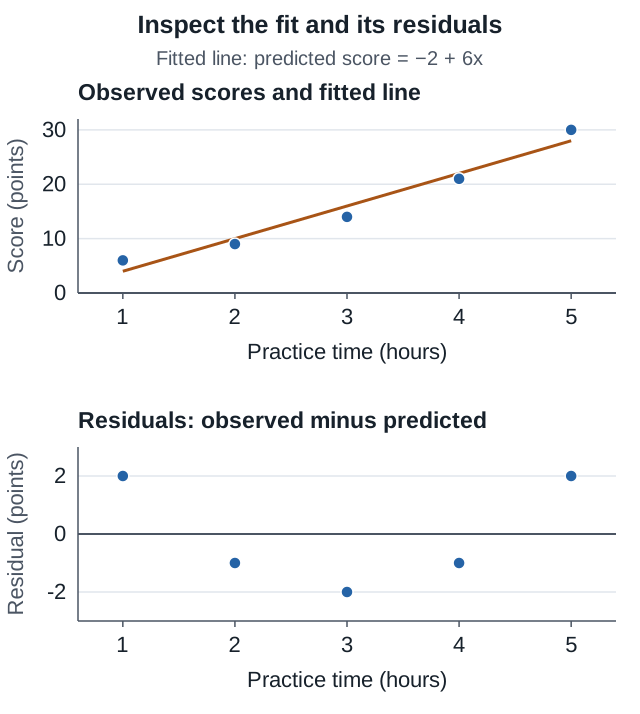
| Practice hours x | Observed score y | Predicted score | Residual y − ŷ |
|---|
| 1 | 6 | 4 | 2 |
| 2 | 9 | 10 | −1 |
| 3 | 14 | 16 | −2 |
| 4 | 21 | 22 | −1 |
| 5 | 30 | 28 | 2 |
The straight-line model underpredicts at the ends and overpredicts in the middle. The residual pattern indicates that the line misses structure. Here r² ≈ 0.9626: a large proportion of variability is accounted for, yet the remaining errors are systematic. Use the plot and the setting along with r². This example diagnoses a linear fit; it does not introduce inference for a regression slope or transformed-model fitting.
Checkpoint 5 — Read a prediction critically
A separate fitted model predicts task score y in points from practice time x in hours: ŷ = 12 + 2.5x. The observed practice times range from 1 to 8 hours. A student who practiced for 4 hours scored 20 points.
- Calculate the predicted score and residual, and say whether the model overpredicted or underpredicted.
- Interpret the slope with its units without making a causal claim.
- Explain the risk in using this line for a student who practiced for 20 hours.
Then use the residual-plot example above to explain why a high r² alone does not establish that a straight-line model is adequate. See Appendix B for the worked response.
APPENDIX A — EXAM PRACTICE AND METHOD CHOICE
A.1 Select the method from the design and response
| Question and data | Method | Main check to remember |
|---|
| One yes/no population proportion | One-proportion z interval or test | Observed counts for an interval; null expected counts for a test |
| Two independent yes/no populations | Two-proportion z interval or equality test | Unpooled interval SE; pooled null SE for an equality test |
| Two categorical variables in one random sample | Chi-square independence test | All expected cell counts greater than 5 |
| Categorical distributions across populations or treatments | Chi-square homogeneity test | Independent random samples or randomized groups |
| One quantitative population mean | One-sample t interval or test | Use s/√n and df = n − 1 |
| Paired quantitative measurements | One-sample t on differences | Define the subtraction order; check the differences |
| Two independent quantitative groups | Two-sample t interval or test | Check each group; use the independent-groups SE |
| Predict a quantitative response from a quantitative x | Descriptive least-squares regression | Check the scatterplot, residuals, and prediction range |
A.2 Write a complete statistical argument
For an inference response, define the parameter, identify the procedure, verify its conditions with the actual setting and numbers, show the statistic or interval, and interpret it in context. When testing, state hypotheses and α and compare the p-value with α. A calculator label alone is not an explanation.
For a data-collection response, name the units and variables, explain the random mechanism clearly enough to reproduce it, control relevant conditions, and state what conclusions the design can support. For a graphical response, connect every description to the measured variables rather than listing vocabulary.
Original short-response practice. Revisit example 7. Before calculating, define p as the proportion of all 4,000 students at that school who support later library hours. Explain how the 200 students could be selected randomly and how nonresponse would be documented. Then state the 10% and large-count checks, construct the interval, and interpret it. Finally, explain why surveying a larger group of self-selected volunteers would not automatically improve representativeness. A complete answer combines design, calculation, interpretation, and a limitation; there is no official scoring rubric for this original exercise.
A.3 Use the current exam format
College Board currently lists the exam for May 11, 2027. The exam uses Bluebook for both sections: 42 multiple-choice questions in 90 minutes and four free-response questions in 90 minutes, each section contributing 50% of the score. Check the linked official exam page for current administration and calculator rules. The 25-question quiz here samples concepts from these notes; it does not reproduce the official section length, shared-prompt structure, or scoring.
Practice entering statistical reasoning in words as well as symbols. Define a parameter before using it, show the relevant tail or interval, and end with a contextual conclusion. After reviewing an error, redo a similar problem without the solution, then explain why each tempting alternative is wrong.
A.4 Set up a calculator calculation
Use cumulative area, not a density height, for a continuous-distribution probability. For a standard-normal test statistic z, the cumulative function Φ(z) gives area to the left using mean 0 and SD 1. An upper-tail test uses 1 − Φ(z); a two-sided test uses 2[1 − Φ(|z|)]. When a calculator asks for bounds, enter the appropriate lower and upper boundaries rather than the confidence level. Device menus differ; retain enough precision and show which tail you used.
For a t test, also enter the correct df and use a t cumulative function, not a normal function. For a normal percentile, the inverse cumulative function uses the area to the left; return the result to the requested measurement units. Before calculation, write the distribution, its parameters, and the requested area or percentile. After calculation, check that a probability lies between 0 and 1 and that your answer addresses the original question.
APPENDIX B — CHECKPOINT ANSWERS AND SELF-REVIEW
B.1 Data summaries and sampling
For checkpoint 1, the median is (4 + 5)/2 = 4.5 minutes. The lower half is 2, 3, 3, 4, so Q₁ = 3. The upper half is 5, 5, 6, 8, so Q₃ = 5.5. Thus IQR = 2.5 minutes. The fences are 3 − 1.5(2.5) = −0.75 and 5.5 + 1.5(2.5) = 9.25 minutes. No observation lies outside them. This convention is stated because software can use different quartile algorithms for small samples.
Volunteers select themselves into the study. Adding more of them does not automatically correct that selection process. A larger volunteer sample may have less random variability while still being systematically unrepresentative.
Check your work: quartiles use the specified convention; IQR and fences have the correct units; no valid observation is deleted merely for looking unusual; sampling bias is distinguished from sample size.
B.2 Probability and a binomial event
For checkpoint 2, n = 4 is fixed, the trials are independent, each has two outcome categories, and p = 0.20 stays constant. Therefore X is binomial. P(X ≥ 1) = 1 − P(X = 0) = 1 − 0.80⁴ = 0.5904. Its mean is np = 0.8 successes. The mean is an average over many repeated four-attempt sets, not the count required in one set.
Check your work: complement means zero successes, not one; 0.5904 is a probability between 0 and 1; 0.8 is an expected count, not a probability of success on one attempt.
B.3 A one-proportion inference response
For checkpoint 3, let p be the proportion of all 3,000 students at this school who support the new opening time. Set H₀: p = 0.50 and Hₐ: p > 0.50. Use a one-proportion z test. The stated simple random sample supplies randomization; 150 ≤ 0.10(3,000) = 300 supports approximate independence. Under H₀, expected successes and failures are both 150(0.50) = 75, so both exceed 10.
The sample proportion is 84/150 = 0.56. Use the null SE, √(0.50 × 0.50/150) ≈ 0.04082. Thus z ≈ (0.56 − 0.50)/0.04082 = 1.470. The upper-tail p-value is about 0.0708. Because 0.0708 > 0.05, fail to reject H₀. The data do not provide convincing evidence that more than half of this school’s students support the new opening time. This result does not establish that support equals one-half or that the proposal has no support.
Check your work: population parameter, hypotheses, null counts, null SE, upper tail, decision, and contextual conclusion are all present. If your calculation is right but your tail or population is wrong, revisit the corresponding step.
B.4 A paired inference response
For checkpoint 4, two measurements belong to each student, so they are dependent within the pair. Let μd be the population mean after-minus-before task-time difference, in seconds, for eligible students. Test H₀: μd = 0 against Hₐ: μd < 0 using one-sample t inference on the differences.
The students were sampled randomly, 12 ≤ 0.10(1,000), and the sample of differences has no strong skewness or outliers. Treat different students’ pairs as independent. Here n = 12 pairs, SE = 6/√12 ≈ 1.732 seconds, t = (−2 − 0)/1.732 ≈ −1.155, and df = 11. The lower-tail p-value is about 0.1363. At α = 0.05, fail to reject H₀: there is insufficient evidence that the population mean after-minus-before difference is below zero.
A negative sample mean is not enough by itself to establish a population decrease. A before-and-after comparison without randomized treatments and an appropriate comparison group also cannot separate practice from other changes over time.
Check your work: the SE uses the SD of differences; n counts pairs; the test uses the lower tail; the conclusion does not claim “no effect” or establish causation.
B.5 Prediction and model limits
For checkpoint 5, ŷ = 12 + 2.5(4) = 22 points. The residual is 20 − 22 = −2 points, so the model overpredicted by 2 points. The slope says that one additional practice hour is associated with an increase of 2.5 points in the predicted score. It does not guarantee that an individual gains those points because of extra practice.
Twenty hours lies outside the observed 1–8-hour range, so the prediction would be extrapolation and the relationship may not continue. In the separate residual-plot illustration, the positive-end/negative-middle pattern signals structure missed by a line despite its high r².
Check your work: prediction and residual are different quantities; the residual sign agrees with the verbal explanation; the slope has points-per-hour units; the prediction range and causal limitation are stated.
B.6 What to do with a mistake
Classify a missed step before rereading: Was it a definition, design, method choice, condition, calculation, or interpretation? Return to that subsection, work a similar case with changed numbers, and then explain the reasoning without the solution visible. Use the checkpoints as a guide to what needs practice, not as an official scoring rubric or evidence that the whole course has been mastered.
These are original HyNote study notes based on College Board’s public AP Statistics framework effective Fall 2026 for the 2026–27 course and May 2027 exam. They are not official College Board materials, a course transcript, or official AP questions, and they are not endorsed by College Board. All examples and practice questions are original teaching exercises. The 25-question quiz is a short practice set, not a full-length exam or a score predictor. Check current official sources for exam rules and use your teacher’s sequence alongside this compact review.


