SAT Math — Problem-Solving and Data Analysis
Purpose: Build the habit of translating a short situation into quantities, choosing a denominator or model, calculating, and checking what the answer means. These original HyNote notes focus on one SAT Math content domain. They are not a complete SAT course, an official question bank, or a full-length adaptive practice test.
Scope and sources: The seven parts follow the skills listed in College Board’s Problem-Solving and Data Analysis overview, checked October 22, 2026. The Math overview describes multiple-choice and student-produced responses; this page’s interactive quiz uses four-choice questions, while the checkpoints ask you to produce and explain an answer. All situations, numbers, charts, questions, and solutions below are invented teaching material. SAT is a trademark of College Board, which does not endorse or produce this guide.
How to study: Open 2 Work in the HyNote Study Loop and read one part at a time. In this page, 1 Map holds Summary and MindMap, 3 Recall holds flashcards, 4 Test holds the Quiz, and 5 Fix holds retries, Comparison, and Formula Sheet. You can select a step directly; you do not need to finish all 50 cards before trying a question. Cover each worked solution, try it yourself, then explain the unit, denominator, or assumption. Attempt that part’s checkpoint in PART 8 before reading Appendix A. Use the corresponding Quiz questions for fresh situations. A calculator can help with arithmetic, but write the relationship first. For exam preparation, use the current calculator policy, official Student Question Bank, and Bluebook practice tests. This pack does not reproduce their questions or scoring.
For deeper explanations of inference, use AP Statistics Notes or Stanford Statistics Notes. For a fuller probability course, use Harvard Statistics 110 Notes. The present guide keeps inference at an interpretation level; it does not require the formal hypothesis tests taught in those courses.
Before you start: check the foundation
You should be comfortable dividing fractions, converting between decimals and percentages, and substituting a value into a formula. Try these three short prompts without looking up the answers: write 0.35 as a percentage; express 18 out of 30 as a percentage; evaluate 2 + 3x when x = 4. Appendix B gives the answers and a route back if a step is unfamiliar.
For one study session, choose one part and its checkpoint rather than trying to memorize the entire pack. Before calculating, write: What is asked? Which whole or group applies? Which units or assumptions matter? After calculating, give a sentence explaining the result. A correct option without a correct setup can be a guess; mark it for review in your own notes even if the page counts it as correct.
PART 1 — RATIOS, RATES, AND UNITS
1.1 Name the whole before dividing
A ratio compares quantities in a stated order. If red:blue = 2:3, the whole has five equal ratio parts. Red is 2/5 of the total, not 2/3 of the total. A proportion equates two ratios measuring the same relationship. Keep the order consistent on both sides.
Worked example 1 — A mixture. A paint mixture has yellow:white = 2:3 and a total volume of 35 liters. How much of each color is used?
Solution: Each ratio part is 35/(2 + 3) = 7 liters. Yellow is 2 × 7 = 14 liters and white is 3 × 7 = 21 liters. Check both the total, 14 + 21 = 35, and the ratio, 14/21 = 2/3. Multiplying 35 by 2/3 would incorrectly treat the total as the white portion.
A unit rate expresses one quantity per one unit of another: dollars per kilogram, kilometers per hour, or people per square kilometer. If a relationship is proportional, y = kx and k is the constant unit rate. A fixed starting fee makes a relationship linear but not proportional: y = 5 + 2x does not pass through the origin.
Worked example 2 — Conversion with units. A runner covers 1.8 kilometers in 6 minutes at a constant speed. Find the speed in meters per second.
Solution: Convert both quantities: 1.8 kilometers = 1,800 meters and 6 minutes = 360 seconds. Speed = 1,800/360 = 5 meters per second. Equivalently, 0.3 kilometers per minute × 1,000 meters per kilometer ÷ 60 seconds per minute = 5 meters per second. Converting only the numerator gives the wrong unit rate.
For area and volume, apply the conversion to every dimension. Since 1 meter = 100 centimeters, 1 square meter = 10,000 square centimeters. Thus 0.6 square meter is 6,000 square centimeters, not 60. Density is count/area, so doubling the area while holding count fixed halves the density.
Before moving on: solve checkpoint 1 in PART 8. Quiz Q1–4 revisit ratios, rates, and conversions.
PART 2 — PERCENTAGES AND CHANGING BASES
2.1 Write the multiplier
A percentage means a fraction out of 100. The relationship part = decimal rate × whole identifies the denominator. For a p% increase, multiply by 1 + p/100; for a p% decrease, multiply by 1 − p/100. Reverse a change by dividing by its multiplier, not by subtracting the same percentage from the new value.
Worked example 3 — Two successive changes. An item originally costs $80. Its price rises 15%, then the new price is discounted 20%. What is the final price and the overall percentage change?
Solution: The marked-up price is 80 × 1.15 = $92. The final price is 92 × 0.80 = $73.60. Overall change = (73.60 − 80)/80 × 100% = −8%, an 8% decrease. Adding +15% and −20% would give −5%, which ignores the changed base. To recover the original price from $73.60, divide by 1.15 × 0.80 = 0.92.
A percentage can exceed 100: 250% of 40 is 100. “150% of the original” means 1.5 times the original; “150% more than the original” means 2.5 times the original. Read the comparison phrase before computing.
Worked example 4 — Percent versus percentage points. A survey’s support rate changes from 18% to 24%. Describe the change in both ways.
Solution: The absolute difference is 24 − 18 = 6 percentage points. The relative increase is (24 − 18)/18 = 1/3, or about 33.3%. A six-percentage-point increase and a 6% increase are not interchangeable. These calculations compare the reported rates; without information on study design and uncertainty, they do not establish why support changed.
Before moving on: solve checkpoint 2. Quiz Q5–7 practice reverse percentages, successive changes, and percentage points.
PART 3 — ONE-VARIABLE DATA AND DISTRIBUTIONS
3.1 Keep the counts attached to the values
The mean is total value divided by number of observations. For a frequency table, multiply each value by its count before summing. A median uses the ordered positions; for an even count, average the two middle values. A mode is a most frequent value, and a range is maximum minus minimum.
Worked example 5 — Combining groups. Twenty students have a mean practice time of 6 hours and another 30 have a mean of 8 hours. Find the combined mean.
Solution: The totals are 20 × 6 = 120 hours and 30 × 8 = 240 hours. Combined mean = (120 + 240)/(20 + 30) = 7.2 hours. The simple average of the two means, 7, incorrectly gives equal weight to unequal groups. The result 7.2 lies between 6 and 8 and is closer to the larger group’s mean of 8.
An unusually large observation can pull the mean upward more than the median. That does not make the mean incorrect; choose the measure that answers the question. Standard deviation measures spread around the mean, in the data’s units. Adding the same constant to every observation shifts the center but leaves spread unchanged. Multiplying every value by c multiplies standard deviation by the absolute value of c. You can reason about these transformations without calculating a long standard-deviation formula. For a concrete comparison, A = 4, 5, 6 and B = 1, 5, 9 both have mean 5. Their deviations from 5 are −1, 0, 1 versus −4, 0, 4, so B has more spread. Here B is exactly four times as far from the common mean at every corresponding position; its standard deviation is four times A’s under the same convention. Equal means do not imply equal spread. Range alone does not generally determine standard deviation.
Try a smaller step: C = 2, 4, 6 is changed to D = 6, 12, 18 by multiplying every value by three. How do mean and standard deviation change? Explain the distance from the mean rather than only naming a rule. Check the bridge answers in Appendix A.
3.2 Read bins without inventing exact values
Worked example 6 — Two histograms. The charts show invented trip times for two groups of 20 students. Bin labels include the lower endpoint and exclude the upper endpoint: 10–<20 means at least 10 but less than 20 minutes.
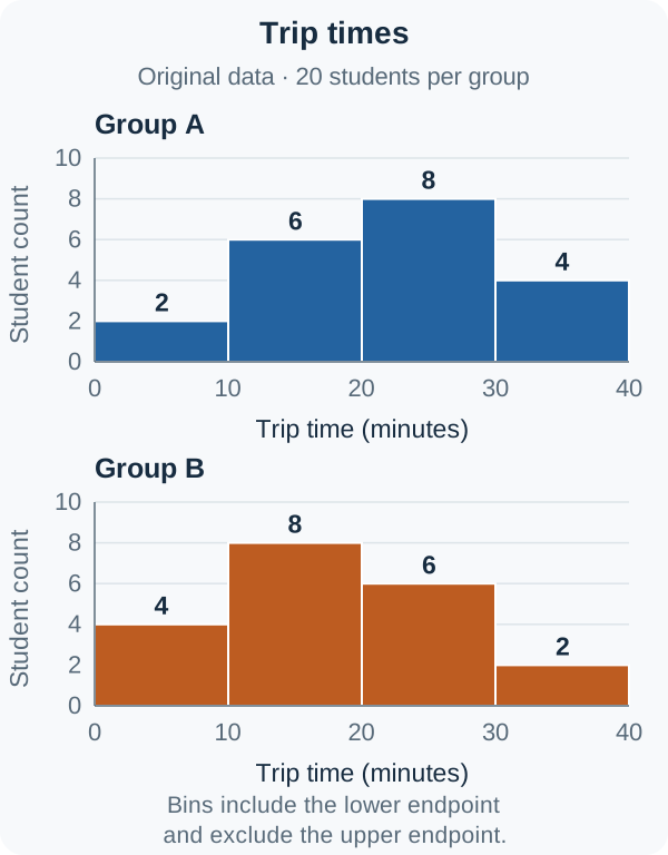
Open this chart to zoom. The matching table below supplies the same data in text.
| Trip time (minutes) | Group A count | Group B count |
|---|
| 0–<10 | 2 | 4 |
| 10–<20 | 6 | 8 |
| 20–<30 | 8 | 6 |
| 30–<40 | 4 | 2 |
| Total | 20 | 20 |
Questions: What fraction of Group A has a trip of at least 20 minutes? Which bin contains each group’s median? Can you calculate either exact mean from the chart alone?
Solution: Group A has 8 + 4 = 12 such trips, or 12/20 = 60%. With 20 observations, the median uses ordered positions 10 and 11. Group A’s cumulative counts are 2, 8, 16, 20, so both positions lie in 20–<30. Group B’s cumulative counts are 4, 12, 18, 20, so both lie in 10–<20. The exact times within the bins are unknown, so neither exact mean is determined. Using bin midpoints would produce an estimate, which must be labeled as an estimate.
Always read axes, interval widths, sample sizes, and endpoints. A bar chart compares categories; a histogram groups numerical values into intervals. These histograms use equal-width bins and counts on the vertical axis. Do not assume every histogram uses the same vertical scale or that equal-looking bars from different sample sizes imply equal percentages. For a box plot, the line inside the box marks the median. The first quartile Q1 and third quartile Q3 mark the box ends; their difference, Q3 − Q1, is the interquartile range (IQR), describing the spread of approximately the middle half of the data. Each quartile interval represents roughly one-quarter of the ordered observations, not an equal distance on the axis. Ties and quartile conventions can affect exact counts. A wider box means a larger IQR; it does not mean a larger sample. Ordinary box widths do not encode sample size unless the display explicitly says so. Read the whisker convention: some plots use the minimum and maximum, while others show outliers separately. A box plot alone generally does not determine an exact mean or standard deviation. Try the new box plots in checkpoint 3b.
Before moving on: solve checkpoint 3. Quiz Q8–12 practice weighted means, frequency tables, outliers, spread, and binned counts.
PART 4 — TWO-VARIABLE DATA AND MODELS
4.1 Separate a prediction from an observation
A scatterplot pairs two numerical variables. Inspect direction, shape, unusual points, and the range of observed x-values. A positive association means larger x tends to accompany larger y; it does not prove x causes y. A linear model written as predicted y = a + bx has a rate of change b, measured in y-units per x-unit. Its intercept a predicts y at x = 0, which may be outside a meaningful range.
Worked example 7 — Prediction and residual. For invented practice data, a proposed model is predicted score = 12 + 3x, where x is practice hours. What is predicted at four hours? If the observed score is 26, what is the residual?
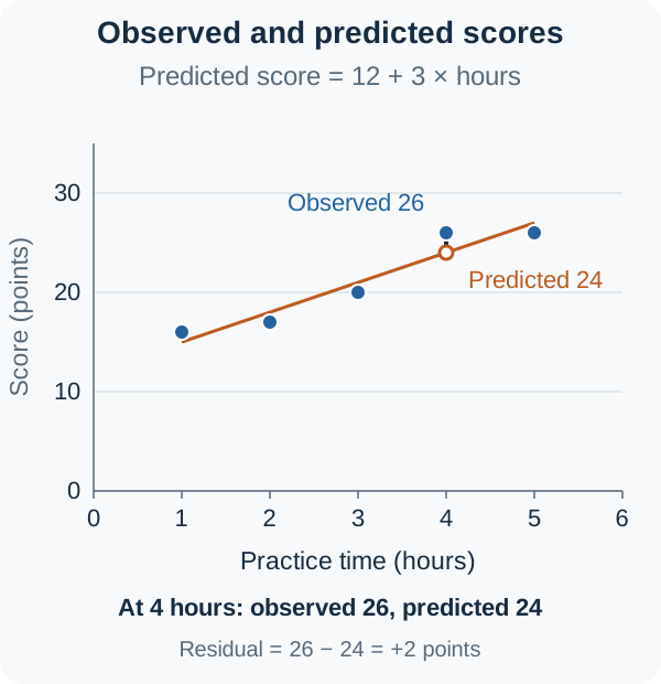
Open this chart to zoom. The matching table below supplies the same data in text.
| Hours x | Observed score | Model prediction | Observed − predicted |
|---|
| 1 | 16 | 15 | 1 |
| 2 | 17 | 18 | −1 |
| 3 | 20 | 21 | −1 |
| 4 | 26 | 24 | 2 |
| 5 | 26 | 27 | −1 |
Solution: At x = 4, prediction = 12 + 3 × 4 = 24 points. Residual = observed − predicted = 26 − 24 = +2 points. The positive residual means the observed point is above the line. The model’s slope is three score points per additional practice hour; it is not a statement that every individual score rises by exactly three. This is a supplied model for practice, not a claim that it is the least-squares line or that the relationship is causal.
Predicting within the observed x-range is interpolation. Predicting far outside it is extrapolation and needs caution: the same relationship may not continue. A model can summarize association while missing curvature or other patterns.
Worked example 8 — Additive or multiplicative growth? One model is y = 100 + 20t and another is y = 100(1.20)^t. What does each assume, and what does the second predict at t = 3?
Solution: The linear model adds 20 units each time t rises by one. The exponential model multiplies by 1.20 each step, a 20% increase based on the preceding value. At t = 3, the exponential prediction is 100 × 1.20³ = 172.8, whereas the linear prediction is 160. If the quantity is a count, 172.8 is a model prediction and could be reported as approximately 173 when whole units are requested. Do not silently round intermediate arithmetic.
Before moving on: solve checkpoint 4. Quiz Q13–16 address prediction, residuals, growth factors, and extrapolation.
PART 5 — PROBABILITY AND CONDITIONAL GROUPS
5.1 Identify the group from which selection occurs
For equally likely individual selections, probability = favorable count / eligible count. A condition changes the eligible group. “A or B” includes either or both unless the question specifies otherwise. Add the counts and subtract the overlap once: P(A or B) = P(A) + P(B) − P(A and B). Mutually exclusive events cannot happen together; independent events have probabilities unchanged by learning that the other occurred. These are different ideas.
Worked example 9 — A two-way table. One of these 80 students is chosen uniformly at random. The categories in each row are exhaustive and non-overlapping.
| Grade | Bikes | Takes bus | Total |
|---|
| Grade 11 | 18 | 32 | 50 |
| Grade 12 | 9 | 21 | 30 |
| Total | 27 | 53 | 80 |
Questions: Find the probability of biking, biking given Grade 12, and Grade 12 given biking.
Solution: P(bikes) = 27/80. Given Grade 12, only those 30 students are eligible, so P(bikes given Grade 12) = 9/30 = 0.30. Given biking, only the 27 bikers are eligible, so P(Grade 12 given bikes) = 9/27 = 1/3. The two conditional questions reverse the condition and generally have different denominators. The joint probability of Grade 12 and biking is 9/80, a third quantity.
Worked example 10 — Without replacement. A bag holds four green and six yellow tokens. Two tokens are drawn uniformly at random without replacement. Find the probability both are green.
Solution: The first probability is 4/10. Given that a green token was removed, three green tokens remain among nine tokens, so the second probability is 3/9. Multiply along that path: (4/10)(3/9) = 2/15. These draws are not independent. With replacement and remixing, the second probability would stay 4/10, giving 4/25 instead.
For another overlap check, suppose 50 members include 20 in chess, 18 in music, and eight in both. The number in at least one is 20 + 18 − 8 = 30, so the probability is 30/50 = 0.60. Adding 20 and 18 alone counts those eight members twice. For a complement, P(not A) = 1 − P(A); “at least one” can often be calculated as one minus “none,” with the correct dependence assumptions.
To read probability notation, let A and B stand for named events; “and” means their overlap, while “given B” restricts selection to B. When P(B) > 0, P(A given B) = P(A and B)/P(B). In the school table, Grade 12 and biking has probability 9/80, and Grade 12 has probability 30/80. Their ratio, (9/80)/(30/80), is 9/30, the same restricted-group calculation used above.
Independence can be checked using P(A and B) = P(A) × P(B). For example, a spinner landing red with probability 0.4 and a separate independent fair coin landing heads have joint probability 0.4 × 0.5 = 0.2. Both events can occur together; independence does not mean “no overlap.” In contrast, a single die roll cannot be both a 1 and a 2. Those two positive-probability events are mutually exclusive, so learning that one occurred changes the other’s probability to zero.
Try a smaller step: Suppose P(A) = 0.5, P(B) = 0.4, and P(A and B) = 0.1. Are the events independent? Are they mutually exclusive? Check both definitions before reading the bridge answers in Appendix A.
Before moving on: solve checkpoint 5. Quiz Q17–20 revisit overlap, conditional denominators, dependent draws, and independence.
PART 6 — SAMPLES, ESTIMATES, AND MARGIN OF ERROR
6.1 Match a statistic to its target population
A population is the full group a question concerns; a sample is the observed subset. A sample statistic estimates an unknown population parameter. Random selection helps support inference to the population from which the sample was drawn, provided coverage, response, and measurement are appropriate. A large voluntary poll can remain biased; increasing the count alone does not repair systematic undercoverage or nonresponse.
Worked example 11 — Estimate a population count. A simple random sample of 100 of a library’s 2,000 adult members includes 58 who prefer extended evening hours. What count of members preferring evening hours does the sample proportion estimate?
Solution: The sample proportion is 58/100 = 0.58. Estimated population count = 0.58 × 2,000 = 1,160 adult members. It is an estimate, not a census result or a guarantee. The target is this library’s adult members, not every resident or all library users worldwide. A random sample’s result can vary even when selection is well designed.
6.2 Interpret uncertainty without overclaiming
Worked example 12 — An estimate with uncertainty. A well-designed random survey reports 54% support with a margin of error of three percentage points at its stated confidence level. What interval is reported, and what does it mean?
Solution: The endpoints are 54% − 3% = 51% and 54% + 3% = 57%. Interpret this as a plausible range for the target population’s support rate under the survey’s method and assumptions. It is not an interval containing 51% to 57% of individual people’s answers, and the margin is not 3% of 54. A stated 95% confidence level describes the long-run coverage of intervals produced by the method under repeated sampling; it is not a claim that 95% of responses are correct. The unknown population proportion is fixed, while the sample and its interval vary. Imagine repeating the entire random-sampling procedure many times and building an interval each time. A method with 95% coverage would capture that same fixed population proportion in about 95% of the intervals over the long run, under its assumptions. It does not promise exactly 95 successes in every batch of 100, nor say that 95% of individuals lie in this percentage interval.
For comparable random-sampling designs at the same confidence level and similar population variability, margin of error decreases approximately as 1/√n. Quadrupling sample size approximately halves it; doubling sample size does not. Holding the data and method fixed, a higher confidence level generally needs a wider interval. Sampling margin of error does not automatically include bias caused by a badly worded question, unrepresentative coverage, or missing responses.
Before moving on: solve checkpoint 6. Quiz Q21–23 address population scope, interval endpoints, and sample-size effects.
PART 7 — WHAT A STUDY CAN SUPPORT
7.1 Random sampling and random assignment do different jobs
Random sampling chooses who enters the sample from a population. Random assignment allocates participating subjects to treatments. The first addresses the scope of population inference; the second helps make treatment groups comparable and supports causal reasoning in a properly conducted experiment. Neither step guarantees a flawless study.
| Design feature | What it helps support | What it does not establish alone |
|---|
| Random sample, observational measurements | Population-level association for the sampled population | A causal effect |
| Random assignment of volunteers | A causal treatment comparison for participants under the study conditions | Representation of an entire population |
| Random sample and random assignment | Broader population inference and a causal comparison, with appropriate implementation | Freedom from nonresponse, noncompliance, or measurement problems |
| Neither | Description of the observed group | General population or causal claims merely from the design |
Worked example 13 — A representative association. Investigators randomly sample students at one school, then record screen time and sleep time without assigning either. Greater screen time is associated with less sleep. What can they conclude?
Solution: With adequate response and measurement, the sample can inform an association among that school’s students. It does not show that increasing screen time causes reduced sleep. Homework load, schedules, or other variables may affect both; the direction of influence may also be uncertain. Random sampling does not turn an observational study into a randomized experiment.
Worked example 14 — An experiment with limited scope. Sixty volunteers are randomly assigned to practice a task with music or in silence. The tasks, timing, and scoring are otherwise comparable, and the music group performs better by an amount supported by the study’s statistical analysis. What is justified?
Solution: Proper random assignment and conduct support a causal comparison of these conditions for the participants. Because the participants volunteered rather than being randomly sampled from all students, the design alone does not establish that the same effect applies to all students. Random assignment makes groups comparable in expectation; it does not guarantee perfectly identical groups in every realized experiment. A simple difference between two sample averages, without considering variation or the analysis, is not automatically convincing evidence.
When judging a claim, identify population, selection, treatment allocation, measurement, and the actual outcome. Watch for a conclusion that changes the population or substitutes causation for association. These are reasoning questions: knowing a formula will not repair an unsupported claim.
Before moving on: solve checkpoint 7. Quiz Q24–25 revisit observational and experimental conclusions.
PART 8 — TRY NEW CHECKPOINTS
Write your setup and explanation before opening Appendix A. These short constructed-response exercises use fresh data and are not official student-produced response questions or a scoring rubric.
- Ratios: A blend uses oats:seeds = 5:3 and weighs 48 grams. Find the mass of each ingredient and explain why 5/3 is not the oats fraction of the total.
- Percentages: A $120 item is discounted 20%. Find the sale price, recover the original price from the sale price, and determine whether raising the sale price by 20% restores $120.
- Data: For 2, 4, 4, 6, 9, find mean and median. If 10 is added to every value, how do the mean, median, and standard deviation change? Then try the separate graph extension 3b below.
- Models: A supplied model is predicted y = 7 + 2.5x. At x = 8, observed y is 24. Find the prediction and residual, with an interpretation of the sign.
- Probability: Of 80 club members, 32 study coding. Twelve of those coders are seniors. Find P(senior given coding) and P(senior and coding). Explain the different denominators.
- Inference: A survey reports 61% with a five-percentage-point margin of error. Give the interval. If sample size rises from 900 to 3,600 under comparable conditions, estimate the new margin of error.
- Claims: A random sample from one town records exercise habits and wellbeing without assigning exercise. Explain the scope of population inference and whether the design proves exercise causes greater wellbeing.
Graph extension 3b — read a new display
The two box plots use a common minutes scale. Here the whiskers explicitly mark minimum and maximum; the diagram does not encode sample sizes. Read the plotted positions before checking the table, which provides the same information in text.
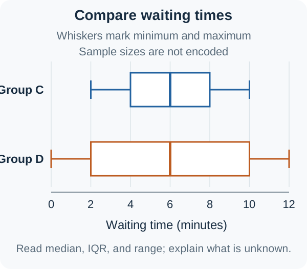
Open this chart to zoom. The matching table below supplies the same data in text.
| Group | Minimum | Q1 | Median | Q3 | Maximum |
|---|
| C | 2 | 4 | 6 | 8 | 10 |
| D | 0 | 2 | 6 | 10 | 12 |
Find both medians, IQRs, and ranges. Which group has more spread in its middle half? Does a longer box establish a larger sample? Can these summaries alone determine either exact mean or exact standard deviation? Explain what is known and what remains unknown, then use the graph-extension answer in Appendix A.
Afterward, use Quiz Q1–4 for ratios/units, Q5–7 percentages, Q8–12 one-variable data, Q13–16 models, Q17–20 probability, Q21–23 inference, and Q24–25 study claims. The 25 questions sample the domain’s skills; they cannot certify mastery of the whole SAT Math section. For an authentic exam-format check, use the current official practice resources linked at the start.
APPENDIX A — CHECKPOINT ANSWERS AND REVIEW
- Total ratio parts = 5 + 3 = 8. Each part weighs 48/8 = 6 grams, so oats weigh 30 grams and seeds weigh 18 grams. The oats share is 5/8 of the whole; 5/3 compares oats with seeds.
- Sale price = 120 × 0.80 = $96. Reverse the discount with 96/0.80 = $120. A 20% rise from $96 gives $115.20; its base is $96, so the equal percentage does not undo the discount.
- Sum = 25, so mean = 25/5 = 5. The middle ordered value is 4. Adding 10 makes mean 15 and median 14; standard deviation is unchanged because every deviation from the mean is unchanged.
- Prediction = 7 + 2.5 × 8 = 27. Residual = 24 − 27 = −3, so the observed value is three y-units below the model prediction. A negative residual does not mean x itself is negative.
- P(senior given coding) = 12/32 = 3/8 = 0.375. P(senior and coding) = 12/80 = 0.15. The condition restricts the eligible group to coders; the joint probability selects from all club members.
- The reported interval is 56%–66%. Multiplying sample size by four approximately divides margin of error by √4 = 2, giving 2.5 percentage points, under the same confidence level and comparable design and variability. This change does not remove systematic bias.
- With appropriate sampling coverage, response, and measurement, the sample can inform an association in that town’s sampled population. Exercise was not randomly assigned; confounding or reverse direction may explain an association. The design does not establish causation or automatically generalize to other towns.
Graph extension 3b — answer
Both medians are 6 minutes. Group C has IQR = 8 − 4 = 4 minutes and range = 10 − 2 = 8 minutes. Group D has IQR = 10 − 2 = 8 minutes and range = 12 − 0 = 12 minutes, so D has greater spread in its middle half. A wider box does not establish a larger sample; sample size is not encoded here. These five-number summaries do not supply the exact observations, so the exact means and standard deviations are not determined. In particular, matching medians do not force matching means, and an IQR comparison alone is not a universal standard-deviation rule.
Bridge practice — answers
For C = 2, 4, 6 and D = 6, 12, 18, mean changes from 4 to 12. Each deviation from the new mean is three times the corresponding original deviation, so standard deviation triples under the same convention. Adding a constant and multiplying by a constant have different effects on spread.
For the probability check, 0.5 × 0.4 = 0.2, which differs from the stated joint probability 0.1, so A and B are not independent. They are not mutually exclusive either, because their overlap has positive probability 0.1. “Dependent” does not mean “mutually exclusive.”
Fix a missed question by naming the error: relationship, base, unit, count, denominator, model, or claim. Rework it without the solution, then try a fresh problem on a later day. If arithmetic was right but the denominator, population, or conclusion was wrong, treat that as a reasoning gap to revisit rather than a minor calculator slip.
APPENDIX B — FOUNDATION CHECK AND NEXT SESSION
The starting answers are 35%, 60%, and 14. For the second, 18/30 = 0.6 = 60%; for the third, multiply first: 2 + 3 × 4 = 14. If these are unfamiliar, use PARTS 1–2 slowly and review basic fraction division, percentage conversion, or substitution before tackling inference. This page is a review and practice guide, not a replacement for instruction in those prerequisites.
To review one skill, first write a setup and answer without notes, then compare the reasoning as well as the result. In 5 Fix, retry missed Quiz questions, open Comparison for sampling versus assignment, or use Formula Sheet for relationships and conditions. A successful repeat of the same question can reflect remembering its answer. Later, change the numbers or use a new official practice question on the same skill, and explain the denominator, units, and conclusion again. Completing cards, getting no recorded misses, or finishing these 25 questions does not by itself establish mastery or predict an SAT score.
Original HyNote study notes, invented examples, and original questions organized around College Board’s public SAT Problem-Solving and Data Analysis skill outline, checked October 22, 2026. This is one Math content domain, not a full SAT course, official question bank, adaptive practice test, or score predictor. SAT is a trademark of College Board; College Board does not endorse or produce this guide. Charts and data are original, and source links identify background specifications rather than authorship of this pack.


